|
December 2010: Ground signatures of ballooning modes: 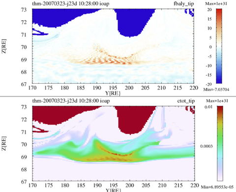
Figure 1: Projection of ballooning structures into the ionosphere. They look like auroral "beads" that are frequently observed, however, they are not simple "blobs" but have some structure. Note that the axes are mislabeled, they should be labeled "geomagnetic longitude" and "geomagnetic latitude" respectively. |
Since we first observed the ballooning mode in OpenGGCM simulations of the March 23, 2007 substorm, we have mapped these structures to the ground. Although we do not know what physical process would create auroral signatures, one can assume that the morphology of the mapped structures resembles that of auroral emissions, regardless of the process. 2010 Fall AGU talk SM54B-04 (tar file) Publication: Nothing yet, planned for proceedings of 2011 Chapman conference. |
|
August 2010: Ballooning modes in the tail: 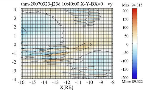
Figure 1: Finger-like structures in the center of the tail current sheet, showing the presence of the classical ballooning mode. The wavelength of the mode is roughly 0.5 RE, consistent with recent Geotail observations (Saito, GRL, 35, L07103, 2008). 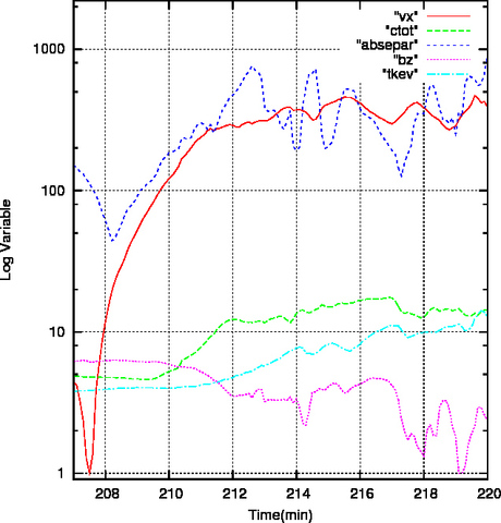
Figure 2: Growth of the axial (KY0) mode. The development of sevaral variables (vx: x-velocity, ctot: current density, absepar: parallel electric field, bz: magnetic field z-component, and tkev: temperature in kV) are shown at the center fo the current sheet. The growth time is of the order of 2 minutes, which is consistent with the the observed growth of some auroral features (Liang et al., GRL, 35, L17S19, 2008), and with the time scale of the explosive growth phase (Ohtani et al., JGR, 97, 19311, 1992). |
Recent global simulations of substorms show that before the onset of near-Earth reconnection the pressure equilibrium in the tail breaks down. This instability has no cross tail variation and is thus not a ballooning mode, and it is also distinct from the tearing mode. Here, we analyze an OpenGGCM simulation run of the March 23, 2007 substorm and find the same instability. Because this mode has no significant cross tail variation associated with it we call it the KY0 mode. Besides the KY0 mode we also find the classical ballooning mode in the simulation. It has a wavelength of ~0.5 RE and is marginally, but sufficiently, resolved as shown by a higher resolution control run. These results suggest a new scenario for the substorm expansion phase onset. During the growth phase magnetic flux is added to the lobes and the plasma sheet thins but remains in equilibrium. When force balance is no longer possible the KY0 instability growths and accelerates plasma tailward. The divergence of the resulting tailward flow reduces the normal magnetic field and thereby makes the current sheet tearing unstable. The tearing mode growths right out of the KY0 mode. The classical ballooning mode grows at the same time and is superimposed on the KY0 mode, but its role in initiating reconnection is still unclear. The growth time of the KY0 mode, ~2 minutes, is both consistent with the notion of an explosive growth phase and with recent ground based observation of the initial growth of auroral arcs before auroral breakup. PPT presentation Movie showing the y-component of the velocity in the tail current sheet just before substorm onset. The finger-like structures are predicted by theory. The wave number ky of these structures matches recent Geotail observations (Saito et al., GRL, 35, L07103) of ~0.5 RE. Movie Same as the previous movie, but for a higher resolution run, showing that the scale of the structures is resolved. Publication: J. Geophys. Res., 115, A00I16, doi:10.1029/2010JA015876, 2010. |
|
December 2010: Flux Transfer Events when the IMF is Dominantly B_y: 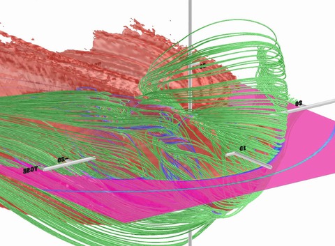
Figure 1: 3D rendering of FTE formation. The red surface is the separatrix separating the closed field lines from the rest. Green field lines are open, blue field lines are closed. The movie corresponding to this figure also shows pink field lines, which are unconnected to the Earth. 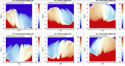
Figure 2: The six panels show a projection of the normal magnetic field component on the magnetopause. The subsolar point is in the center. The mapping algorithm is not perfect, in particular near the cusps, but sufficient to show the FTEs. The six panels correspond to negative IMF By (top row) and positive IMF By (bottom row), summer dipole tilt (left column), no dipole tilt (middle column), and winter dipole tilt (right column). FTEs always form near the subsolar region. They move towards dawn for -By/summer and +By/winter or dusk for +By/summer and -By/winter. For small or zero dipole tilt they randomly move either way. The Movie shows this more clearly. |
Simulation of the May 8, 2004 FTEs observed by Cluster and Double Star (DS1) show that the OpenGGCM can reproduce them quite well. Specifically, the polarity, cadence, duration, and amplitude of a series of FTEs can be reproduced when the OpenGGCM is driven by measures SW/IMF data. |